The Gideon visual SLAM pipeline for the warehouse of the future

Since the dawn of humanity, we have relied on our eyes to orient ourselves in the world: we look at the stars and the sun, at the mountains and rivers to create maps and understand where we are. Throughout history, many technological breakthroughs were inspired by nature; for example, convolutional neural networks were influenced by the human visual cortex [1], [2]).

We at Gideon are no strangers to turning to nature for inspiration when developing our autonomous mobile robots. And this is especially true when it comes to our goal of developing human-like perception for our robots. A goal we aim to achieve by developing a vision-based pipeline for simultaneous localization and mapping (SLAM).

An ancient map of the Bornholm island in Denmark discoverd during the excavation of a Neolithic shrine at Vasagård in 2016. The stone depicts topographical details of the land on the island as it was between 2700 and 2900 BC.

Why robot vision?

You might wonder why we primarily rely on vision since multiple kinds of sensors are available.

This is because we want our robots to navigate safely and responsibly in indoor and outdoor environments, regardless of the time of the day and whether it is raining, snowing, or sunny.

And our Vision Module helps us achieve just that. It provides reliable information in environments where other sensors, like GPS, might not provide enough information to enable precise and safe localization and mapping. Vision excels in many environments such as indoor warehouses or even metro stations, airports, and other spaces, even for the purpose of virtual reality.

After all, the Perseverance is able to accurately navigate on the surface of Mars, relying on vision as the primary source of information!

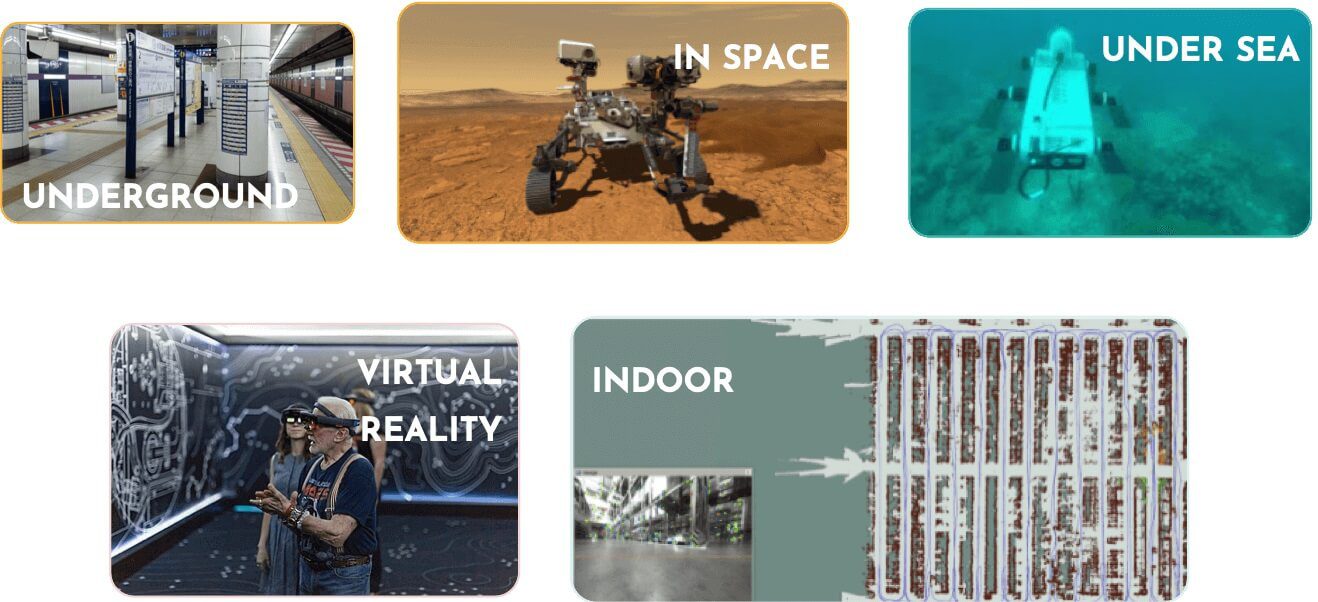
The applications of visual SLAM: underground, in space [3], undersea [4], in augmented & virtual reality, and in indoor environments.

Why are SLAM and autonomous mobile robots a perfect fit for warehouses?

Let’s get down to business and see why SLAM and autonomous mobile robots (AMR) work well together in warehouses. We at Gideon are developing AMRs to help us share the load by doing the physically hard, repetitive, dull, and messy jobs while keeping the workers safe and allowing them to focus on other “smarter” tasks.

Say we want to tell our robot, which we’ll call Ozzy (or a fleet of robots): “Hey Ozzy, unload this trailer and take all the cargo to warehouse area A”. To know where warehouse area A is, the robot first needs to have some kind of a map of the warehouse or the outdoor areas such as parking. So, let’s start with that.

Mapping: building Rome (or Dubrovnik) in real time

How do we build a map from a sequence of images that our robot Ozzy perceives? Or, to be more precise: how do we go from this 2D world of images and pixels into our 3D and find out that we are 30m away from warehouse area A, and we need to rotate 60 degrees to get there?

There are many ways to tackle this problem. There are different map representations (image-based or 3D structure-based), and there are different methods (both deep learning-based and traditional computer vision methods). They can generally be divided into a few stages:

i) image parsing & feature extraction,
ii) feature matching,
iii) pose estimation and
iv) map update.

Please note that some stages may be combined into a single component. Each of these stages deserves its own blog post; we will give a bird’s eye overview of the visual SLAM components.

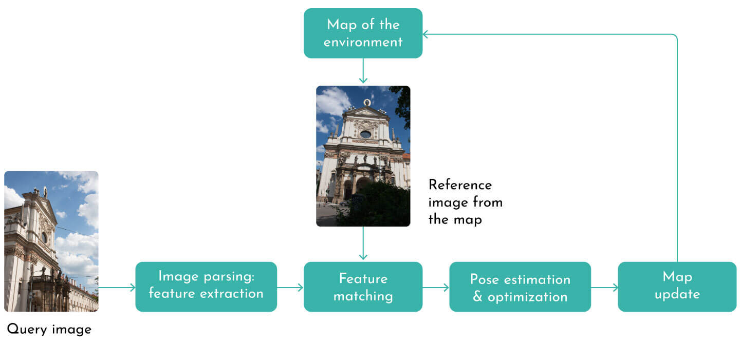
The SLAM mapping pipeline scheme, image credit: Kornia computer vision library

Image parsing

We start with images, so let’s see how to parse them and find out what’s unique and useful about them.

One efficient and often used method is to extract global image descriptors [5], [6], [7], [8], [9]. These global descriptors are convenient to determine the agent’s position quickly.

Say you already have a map of the Dubrovnik old city and an image (e.g. depicting the Jesuit Stairs), and you want to quickly determine where exactly in Dubrovnik you are?

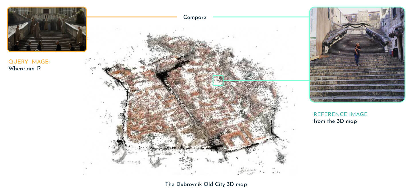
Visual localization with global descriptors. Having an arbitrary image taken in the Dubrovnik Old City, e.g., the Game of the Thrones scene, determine where the scene was filmed and visit the landmark (the Jesuit Stairs).

These global descriptors can be seen as numerical one-sentence image descriptions telling us something like, “Oh, hey, there’s a mountain in this image or a cathedral or a shopping center”.

In order to compute this global descriptor, we need to find out what makes this image different from other (nearby) images. This is actually a ranking problem, often optimized with a contrastive (triplet) loss, where we want our query image Iq to be closer to some image describing the same scene (a positive example Ip), than to some other image (a negative example In):

distance(Iq,Ip) − distance(Iq,In) < margin

This problem can be solved with traditional bag-of-visual-words methods [10], [11], [12], [13] of with deep learning approaches [5], [6], [7], [8], [9]. For learning-based approaches, we need the so-called “time machine data”, i. e., images captured at different times of day, seasons, and weather conditions to train the model.

In general, the network architecture is usually composed of two parts: an encoder that captures visual information and then pooling, which creates a digest, a one-sentence description of the scene.

As outlined above, the global descriptors can help us quickly narrow down where we are in the environment. But we need to do a little better than that to move objects around a warehouse efficiently. This is where local feature extraction comes into play.

Local feature extraction

So what makes for a good local feature? Essentially, we want to find something that we can easily find in other images, making for a good correspondence.

Obviously, we also want to disregard moving objects like vehicles or people. They tend to move around, so they are not vital for describing the scene’s geometry. We are looking for static features – similarly as our ancestors once looked at the stars or mountain peaks. Another thing to keep in mind is the robustness: you want to be able to detect this window in another image, no matter if it’s daytime, nighttime, snowing, or raining.

So, how do you capture this information? What makes a mountain peak or a window, regardless of the conditions around it?

Traditionally this has been solved with handcrafted features like SIFT [14], [15], [16], which still work pretty well in practice in some cases (e.g., in daytime scenarios). But to really achieve robustness, we need to learn how to extract these features, which would make for good correspondences.

As the world is not static – weather and seasons change, the scene’s geometry also changes, our SLAM solution has to be robust to such changes. Image credit: the visual localization benchmark

What better way to do that than to learn on a pair of images? So for training data, you need pairs of images that partially observe the same scene and optionally known correspondences between them (some methods do not require explicit correspondence, like R2D2 [17] ).

Then we can minimize the matching loss between the corresponding features.

min d(f(I_q), f(I_r))

Here, we use the f(I), we denote the network output (entire feature maps or just sparse features) for the image I, whereas d(⋅,⋅) denotes some kind of distance metric (e.g., correlation, or ℓ2 distance).

The architecture is usually composed of encoder and decoder heads (decoders) that predict feature locations (keypoint pixels) and their descriptions. They tell us if something is the top of the cathedral, a window corner, or a text on some monument.

We often predict some kind of score that tells us how certain we are that there is a feature at that specific location. Some popular solutions include SuperPoint [18] or R2D2 [17].

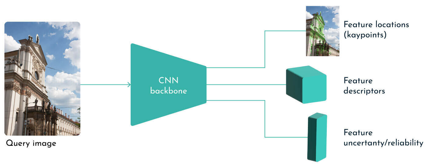
Learning-based feature extraction at inference time.

Image matching

Now that we know how to extract what’s relevant in the images, let’s estimate the movement of the pixels.

Image matching for pose estimation in an outdoor scenario.

Matching can be done traditionally with the nearest neighbor search in the descriptor space, which can be further sped up by using KD trees [19], [20], [21], [22].

However, in the deep learning domain, the transformers [23], [24], [25], [26] have emerged as the defacto standard for set matching.

The transformers are tailor-made for matching sets, no matter if you want to match a set of words in Chinese to English; or a set of bounding box predictions to a set of ground truth objects. Or perhaps, like in this use case, a set of features in the query image to a set of features in the reference image.

Self-attention

This is what the SOTA methods like LoFTR [26] and SuperGlue [25] are actually doing in a very clever way. And here, we’re going to look at nature for inspiration once more – when faced with such ambiguous situations, where we have repetitive patterns like a checkerboard, for example, we look for a nearby object, which can help us gain some insight into how the camera has moved around. This idea of looking inside a single image to gain context is called self-attention.

Just like we might ask ourselves how much the word “SLAM” is important for translating the word “future” within the sentence “Visual SLAM pipeline for the warehouse of the future“, we might also ask ourselves the next question. How much is the feature on the notebook in the image below important for matching other features on the checkerboard?

And we do so by classic attention pooling so, queries Q, keys K and values V both come from the same distribution (the same image), and we do weighted attention pooling of values, depending on the queries and keys.

Attention(Q,K,V) = softmax (Q⋅KT) ⋅ V

The importance of context for matching. When faced with matching such repetitive patterns (e.g., checkerboard), we humans look for context to help us resolve ambiguities (e.g., the notebook placed over the checkerboard). Image credit: SuperGlue

Cross-attention

Another, maybe more straightforward, idea in this setting is cross-attention. With cross-attention, we use the features (keypoints) from one image as queries to activate the most similar features in the other image as values. This is also done via classic attention pooling. Finally, we perform this matching by alternating self and cross attention layers.

Camera pose estimation

So when we have our matches, pairs of points, we can then estimate the camera movement between the two images via rotation R and translation t.

This part is in most of the SOTA approaches [27], [25] still done in a traditional way with optimization algorithms inside a RANSAC loop, without neural networks (although there have been some attempts to estimate pose in such a way but with poor generalization properties and lower performance [28]).

Let’s make a quick overview. When you think about it, there are 6DoF for this problem: 3 for rotation (e.g., yaw, pitch, and roll) and 3 for translation (in x, y, and z directions). Each pair gives us 2 equations – or constraints, so we need at least 3 pairs of points, and this is called the P3P problem [29]. There are well-known solutions for this problem: Ceres from Google, GTSAM, or PoseLib.

Localization: bringing it all together

We now have our 3D map of the world (you can look at it as Theseus’s ball of thread, the so-called Ariadne’s string) and an image of our current surroundings. So we first use global localization to compute a global descriptor, or say “one sentence that describes the scene”, and compare this descriptor to all global descriptors in a scene – this helps us quickly identify where we are.

Then we do fine matching between our query image and the selected candidates to obtain the matches and then compute the pose where we are on the map.

Long-term visual localization – a real-world use case

Below you can see how this works in action for an outdoor scenario. The video shows a fine example of a real-world, long-term localization in adversarial conditions.

Remember our robot Ozzy whose mission is to help us share the load? Well, on one sunny day, he went for a drive on a lovely parking lot he had never visited and created a 3D map of it.

This map was then shared with a fellow robot Marija. Marija “decided” to explore this parking lot one month later. But, she was able to get there in the early evening, and this time it was raining like cats and dogs.

By using Gideon’s state-of-the-art visual SLAM technology, she was able to correctly estimate her position in the map created by a fellow robot Ozzy.

This shows that the visual SLAM (mapping and localization) is reliable for real-world use cases and, equally important – it is scalable. Once created, the 3D map of the world can be shared with a fleet of robots. These robots can then work side-by-side with humans in building warehouse logistics solutions of the future (to boldly go where no robot has gone before…).

Conclusions and takeaways: ready player one?

Now that we have shown the major components of the visual SLAM pipeline in action, we draw the following conclusions:

• • visual SLAM is vital for automating physically demanding tasks (like material handling in warehouses); or for space exploration and augmented reality
• • visual SLAM is the most natural way to mapping and localization, the way we humans used to map the world and orient ourselves
• • to have safe and robust localization working at night, rain, snow, sunrise, or dusk, we need to have a robust pipeline, and this is where deep learning comes into the game
• • having good data and well-calibrated sensors (cameras) is just as important as the algorithms performing the actual localization

References

[1] D. H. Hubel and T. N. Wiesel, “Receptive fields, binocular interaction and functional architecture in the cat’s visual cortex,” The Journal of physiology, vol. 160, no. 1, pp. 106–154, Jan. 1962.

[2] Y. LeCun, B. E. Boser, J. S. Denker, D. Henderson, R. E. Howard, W. E. Hubbard, and L. D. Jackel, “Backpropagation applied to handwritten zip code recognition,” Neural Comput., vol. 1, no. 4, pp. 541–551, 1989.

[3] J. N. Maki, D. Gruel, C. McKinney, M. A. Ravine, M. Morales, D. Lee, R. Willson, D. Copley-Woods, M. Valvo, T. Goodsall, J. McGuire, R. G. Sellar, J. A. Schaffner, M. A. Caplinger, J. M. Shamah, A. E. Johnson, H. Ansari, K. Singh, T. Litwin, R. Deen, A. Culver, N. Ruoff, D. Petrizzo, D. Kessler, C. Basset, T. Estlin, F. Alibay, A. Nelessen, and S. Algermissen, “The mars 2020 engineering cameras and microphone on the perseverance rover: A next-generation imaging system for mars exploration,” Space Science Reviews, vol. 216, no. 8, p. 137, Nov. 2020.

[4] B. Joshi, N. Vitzilaios, I. Rekleitis, S. Rahman, M. Kalaitzakis, B. Cain, J. Johnson, M. Xanthidis, N. Karapetyan, A. Hernandez, and A. Quattrini Li, “Experimental comparison of open source visual-inertial-based state estimation algorithms in the underwater domain,” 2019, pp. 7227–7233.

[5] R. Arandjelović, P. Gronat, A. Torii, T. Pajdla, and J. Sivic, “NetVLAD: CNN architecture for weakly supervised place recognition,” in IEEE conference on computer vision and pattern recognition, 2016.

[6] S. Hausler, S. Garg, M. Xu, M. Milford, and T. Fischer, “Patch-NetVLAD: Multi-scale fusion of locally-global descriptors for place recognition,” in Proceedings of the IEEE/CVF conference on computer vision and pattern recognition (CVPR), 2021, pp. 14141–14152.

[7] F. Radenovic, G. Tolias, and O. Chum, “CNN image retrieval learns from BoW: Unsupervised fine-tuning with hard examples,” in Computer vision – ECCV 2016 – 14th european conference, amsterdam, the netherlands, october 11-14, 2016, proceedings, part I, 2016, vol. 9905, pp. 3–20.

[8] J. Revaud, J. Almazán, R. S. Rezende, and C. R. de Souza, “Learning with average precision: Training image retrieval with a listwise loss,” in 2019 IEEE/CVF international conference on computer vision, ICCV 2019, seoul, korea (south), october 27 – november 2, 2019, 2019, pp. 5106–5115.

[9] A. Torii, R. Arandjelovic, J. Sivic, M. Okutomi, and T. Pajdla, “24/7 place recognition by view synthesis,” in IEEE conference on computer vision and pattern recognition, CVPR 2015, boston, MA, USA, june 7-12, 2015, 2015, pp. 1808–1817.

[10] H. Jégou, M. Douze, C. Schmid, and P. Pérez, “Aggregating local descriptors into a compact image representation,” in The twenty-third IEEE conference on computer vision and pattern recognition, CVPR 2010, san francisco, CA, USA, 13-18 june 2010, 2010, pp. 3304–3311.

[11] J. Philbin, O. Chum, M. Isard, J. Sivic, and A. Zisserman, “Lost in quantization: Improving particular object retrieval in large scale image databases,” in 2008 IEEE computer society conference on computer vision and pattern recognition (CVPR 2008), 24-26 june 2008, anchorage, alaska, USA, 2008.

[12] J. Sivic and A. Zisserman, “Video google: A text retrieval approach to object matching in videos,” in 9th IEEE international conference on computer vision (ICCV 2003), 14-17 October 2003, Nice, France, 2003, pp. 1470–1477.

[13] F. Perronnin, Y. Liu, J. Sánchez, and H. Poirier, “Large-scale image retrieval with compressed fisher vectors,” in The twenty-third IEEE conference on computer vision and pattern recognition, CVPR 2010, San Francisco, CA, USA, 13-18 June 2010, 2010, pp. 3384–3391.

[14] D. G. Lowe, “Object recognition from local scale-invariant features,” in Proceedings of the seventh IEEE international conference on computer vision, 1999, vol. 2, pp. 1150–1157 vol.2.

[15] R. Arandjelović and A. Zisserman, “Three things everyone should know to improve object retrieval,” in 2012 IEEE conference on computer vision and pattern recognition, 2012, pp. 2911–2918.

[16] M. Calonder, V. Lepetit, C. Strecha, and P. Fua, “BRIEF: Binary robust independent elementary features,” in Computer vision – ECCV 2010, 2010, pp. 778–792.

[17] J. Revaud, C. R. de Souza, M. Humenberger, and P. Weinzaepfel, “R2D2: Reliable and repeatable detector and descriptor,” in Advances in neural information processing systems 32: Annual conference on neural information processing systems 2019, NeurIPS 2019, december 8-14, 2019, Vancouver, BC, Canada, 2019, pp. 12405–12415.

[18] D. DeTone, T. Malisiewicz, and A. Rabinovich, “SuperPoint: Self-supervised interest point detection and description,” in 2018 IEEE conference on computer vision and pattern recognition workshops, CVPR workshops 2018, Salt Lake City, UT, USA, June 18-22, 2018, 2018, pp. 224–236.

[19] D. G. Lowe, “Distinctive image features from scale-invariant keypoints,” International Journal of Computer Vision, vol. 60, no. 2, pp. 91–110, Nov. 2004.

[20] M. Muja and D. Lowe, “Fast approximate nearest neighbors with automatic algorithm configuration.” in VISAPP 2009 – Proceedings of the 4th International Conference on Computer Vision Theory and Applications, 2009, vol. 1, pp. 331–340.

[21] J. Johnson, M. Douze, and H. Jégou, “Billion-scale similarity search with GPUs,” CoRR, vol. abs/1702.08734, 2017.

[22] T. Sattler, B. Leibe, and L. Kobbelt, “Efficient amp; effective prioritized matching for large-scale image-based localization,” IEEE Transactions on Pattern Analysis and Machine Intelligence, vol. 39, no. 9, pp. 1744–1756, 2017.

[23] A. Vaswani, N. Shazeer, N. Parmar, J. Uszkoreit, L. Jones, A. N. Gomez, L. Kaiser, and I. Polosukhin, “Attention is all you need,” in Advances in neural information processing systems 30: Annual conference on neural information processing systems 2017, December 4-9, 2017, Long Beach, CA, USA, 2017, pp. 5998–6008.

[24] N. Carion, F. Massa, G. Synnaeve, N. Usunier, A. Kirillov, and S. Zagoruyko, “End-to-end object detection with transformers,” in Computer vision – ECCV 2020 – 16th European conference, Glasgow, UK, August 23-28, 2020, proceedings, part I, 2020, vol. 12346, pp. 213–229.

[25] P.-E. Sarlin, D. DeTone, T. Malisiewicz, and A. Rabinovich, “SuperGlue: Learning feature matching with graph neural networks,” in 2020 IEEE/CVF conference on computer vision and pattern recognition, CVPR 2020, Seattle, WA, USA, june 13-19, 2020, 2020, pp. 4937–4946.

[26] J. Sun, Z. Shen, Y. Wang, H. Bao, and X. Zhou, “LoFTR: Detector-free local feature matching with transformers,” in IEEE conference on computer vision and pattern recognition, CVPR 2021, virtual, june 19-25, 2021, 2021, pp. 8922–8931.

[27] P.-E. Sarlin, A. Unagar, M. Larsson, H. Germain, C. Toft, V. Larsson, M. Pollefeys, V. Lepetit, L. Hammarstrand, F. Kahl, and T. Sattler, “Back to the feature: Learning robust camera localization from pixels to pose,” in IEEE conference on computer vision and pattern recognition, CVPR 2021, virtual, june 19-25, 2021, 2021, pp. 3247–3257.

[28] A. Kendall, M. Grimes, and R. Cipolla, “PoseNet: A convolutional network for real-time 6-DOF camera relocalization,” in 2015 IEEE international conference on computer vision, ICCV 2015, Santiago, Chile, December 7-13, 2015, 2015, pp. 2938–2946.

[29] M. Persson and K. Nordberg, “Lambda twist: An accurate fast robust perspective three point (P3P) solver,” in Proceedings of the european conference on computer vision (ECCV), 2018.